Single Point Mutation
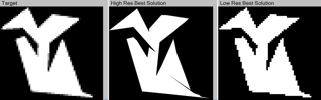
The above image shows three pictures. The first is the target image, which is only 60x60 pixels. The second picture shows the solution found in high resolution, and the third image shown the solution found in low resolution. I find that the final solution has great similarity to the target, although it is far from perfect. The high resolution image has very thin 'spikes' of black that survive because they have no effect on the low resolution image. These results were generated using the single point mutation algorithm, which uses only 1 polygon, and changes, inserts, or removes just 1 point per mutation. The mutation function code for this algorithm is shown below.
The function OutgoingForPoint returns mutation related to a given polygon point in the current solution. We collect mutations for each existing points and intertwine these. The intertwine function allows us to turn a list of enumerables into a single enumerable. It is different from just concatenating each enumerable, in that it is more fair in the order in which the enumerable return values. Given the enumerables {a,b,c} and {1,2,3}, intertwining both would lead to {a,1,b,2,c,3}.
The first mutation that OutgoingForPoint returns is one which removes the given point. The mutations that follow relate to changing the location of the given point, and inserting a new point right behind the given point.
Moving Points
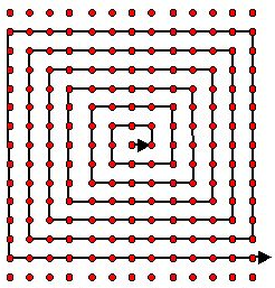
Points are moved by sliding them over a spiral. The simple discrete spiral is chosen so that it does not skip any pixels. The spiral's length is chosen so that is covers the entire target image. To increase performance I evaluate the spiral in a lazy manner, and cache the results.
In a large image, the spiral becomes very large. This leads to very small mutations. Small mutations are bad because they cost an evaluation and can lead to only a slight increase in fitness. This small-step problem is solved by moving over the spiral in a psuedo-random manner. The algorithm is initialized with a constant seed so I get consistent results throughout multiple runs.
For the spiral movement I set the following rules:
1. Pixels close to the spiral's origin have a high chance of being hit early.
2. Every pixel is hit exactly once.
The initial solution I used was very slow. It produces unique spiral locations by selecting a location index according to some destribution, and disregarding the location if it was already produced. This satisfied condition 2. The distribution has a high chance of returning low numbers, so that condition 1. is satisified. Because the distribution tends to return low indices, many of the same indices are returned. It can take extremely long before all the high locations have high been selected. The code for the initial solution is shown below.
A fast integer list, almost constant time removal, indexing and construction.
What I needed to solve the problem of duplicate indices, was a function that would initially map every index back onto itself, but that would never return the same value twice. I settled on using an integer list, that would map integers by using the given integer as an index on itself, and then removing the returned element. The following code displays how we use the list to map integers to integers. We initialized the list using "ListUtil.FromTo(0,count);"
The list should have the following performance characteristics. Constructing the list takes constant time. Removing elements and indexing should be fast, preferably constant time. The solution that worked was similar to just a linked list, but optimized using some specific properties. The list is ordered and without duplicates, so uninterupted sequences in the list can be represented by their first and last element. Such a representation has constant access time, and can be used to construct the initial list quickly, as is done in line 3 of the above code. Removing an element from an integer sequence is done by creating two new sequences and lazily concatenating them. Removing multiple indices in this way can create a binary tree with integer sequences at the leafs, and concatenation operations at the nodes. Removing many indices may create a large tree, which has slow access and remove operations. The trick here is that we can simplify the tree when enough neighbouring indices are removed.
Here follows an example. I'll represent an integer sequence by 1..10. And list concatenation by ",". The balancing of the tree is of minor important so I'll leave out any "()".
We initialize the list: 1..10.
3 is removed: 1..2,4..10
1 is removed: 2,4..10
7 is removed: 2,4-6,8-10
2 is removed: 4-6,8-10
Removing 3 adds two extra nodes to the list, slowed it down. Removing 1 however doesn't add nodes to our list because 1 is at the edge of the sequence 1..2. Removing 7 again decreases performance. Finally 2 is removed which increases performance.
This data structure is perfectly suited for our purpose, because the distribution we use tends to return the same low numbers! The code for removing elements from our data structure is shown below.
